Reversible Data Hiding (Ni et al., 2006)
Ni and colleagues propose reversible data hiding: embedding a message in an image while allowing the original image to be recovered without distortion after extraction. Their method shifts part of the image’s brightness histogram and uses the space it creates to carry bits. The authors motivate exact restoration through medical diagnosis, law enforcement, remote sensing and precision experiments, where permanent changes to the original data can matter. They seek message capacity, small image changes and short execution time together. Zhicheng Ni, Yun-Qing Shi, Nirwan Ansari, and Wei Su, Reversible Data Hiding (2006).
Why must the decoder recover the original image too?
Data hiding places a message inside cover media, the object carrying it. Here the cover is an image, and the altered result is the marked image. Extracting the message alone can leave permanent pixel changes. Section I identifies exact recovery as a separate requirement for applications with legal or precision needs.
The authors distinguish this requirement from hiding changes from human vision. Replacing low-order pixel bits loses their original values. Rounding during transforms can also lose information. A reversible rule must preserve enough information to undo its changes, including any ambiguity created during embedding. The decoder therefore produces both the message and the original image.
Why choose a histogram peak and an empty brightness level?
A histogram counts how many pixels have each brightness value. An 8-bit grayscale image has values from 0 to 255. A peak is a value with a maximum count; a zero point is an unused value. Section II-A chooses the peak because its population determines how many bits can be embedded with a single pair.
The zero point supplies room to shift occupied values without merging their original meanings. The method works directly in the spatial domain, meaning pixel values rather than transform coefficients. Section II-G attributes its low computational load to histogram generation, searches, scans and unit changes, without a transform. Figure 1 labels the peak and zero in Lena’s original histogram.
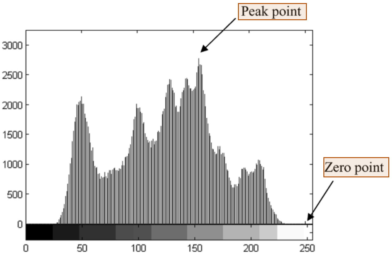
Ni et al. (2006), Figure 1. Peak and zero-point labels.
How does shifting create room for message bits?
Section II-A first empties the brightness level adjacent to the peak. With peak p below zero z, insertion follows these steps:
- Count brightness values and select the peak and zero.
- Increase pixels strictly between them by one, leaving
p + 1empty. - Scan peak pixels in a fixed order; leave each at
pfor bit zero or move it top + 1for bit one.
For original value x and message bit b, the rule is:
x = p:       marked value = p + b
p < x < z:   marked value = x + 1
otherwise:   marked value = x
Take twelve illustrative pixels in scan order: 150, 151, 152, 152, 153, 154, 154, 154, 154, 155, 156, 158. With peak 154 and zero 159, shift 155 through 158 up by one, then embed bits 1, 0, 1, 1 in the four peak pixels, giving 155, 154, 155, 155. Reading 154 as zero and 155 as one recovers those bits; subtracting one from marked values 155 through 159 restores every original pixel.
Why save the positions of pixels at an occupied minimum?
Some histograms have no unused brightness level. Section II-B replaces the zero with a minimum, a value assumed by the fewest pixels. Those pixels would become ambiguous when the shifted range reaches that value. The authors record their coordinates and original brightness as overhead, meaning restoration information carried with the message. Extraction uses these records to restore the minimum pixels.
Equation (1) subtracts this cost from the peak population:
C = h(p) - OHere h(p) is the peak’s pixel count, O is overhead in bits, and C is pure payload, the message capacity after bookkeeping. An empty minimum has no pixel positions to save. The authors use this net capacity when deciding whether another pair is needed.
How does extraction distinguish bits from shifted pixels?
The decoder knows the chosen peak and minimum and scans in the embedding order. For a zero above the peak, marked values at p mean bit zero; values at p + 1 mean bit one. The original intervening pixels have already moved beyond that adjacent level, so they retain separate values.
Section II-C then subtracts one from marked values above the peak through the minimum. This merges the split peak and reverses the range shift. Saved coordinates restore occupied-minimum pixels afterward. Directions reverse when the minimum is below the peak. Figure 5 separates message extraction, the inverse shift and minimum restoration. The original image is an output rather than an input to decoding.
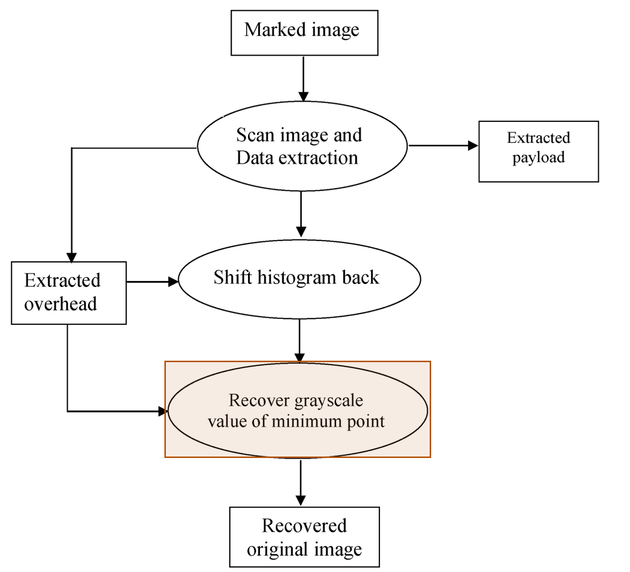
Ni et al. (2006), Figure 5. Restoring the minimum’s grayscale value.
How can several pairs increase capacity without overlapping shifts?
If the required message exceeds pure payload, Section II-B3 adds peak/minimum pairs. Its pseudocode describes three minima in brightness order. It searches the outside intervals for peaks and the intervals between minima for ordered peak candidates. For each minimum, it chooses the candidate with the larger histogram count, then applies the single-pair rule.
This arrangement divides the brightness range into separate shift regions. Extraction repeats the corresponding inverse operations for each pair. Figure 4 increases the pair count until pure payload is sufficient or the allowed count is exhausted. The authors caution that their particular selection may be suboptimal for capacity relative to marked-image quality; they present it as an implementation of the multiple-pair method.
Why restrict pixel changes to one brightness level?
Section II-E derives an image-quality bound from the unit shift. Mean squared error, or MSE, is the average squared difference between original and marked pixels. If every pixel changes by at most one, MSE is at most one. Peak signal-to-noise ratio, or PSNR, expresses this error relative to the brightness range in decibels, written dB.
For the authors’ grayscale setting, Equation (2) gives:
MSE <= 1
PSNR = 10 * log10(255 * 255 / MSE)
PSNR >= 48.13 dB
The authors report experimental support for this bound. Section II-F ties capacity to variation in histogram counts: peaks supply bit positions, while small minima reduce restoration overhead. An exactly horizontal histogram is their stated failure case.
All parts of the method
The encoder counts brightness values, selects peak/minimum pairs, accounts for restoration records and opens adjacent levels through shifts. It embeds the message and overhead into the peak pixels. The decoder reads the split peaks in the agreed order, reverses the shifts and restores occupied minima from their records. Pair parameters and scan order connect the two procedures; the original cover image is recovered at the end.
What experiments did the authors run?
The authors test capacity and quality on common, medical, texture, aerial and CorelDRAW images, illustrate a flat-histogram failure, measure execution time and compare reversible methods.
Common images
Section III uses two peak/minimum pairs for embedding and extraction throughout the image experiments. Tables I–V report pure payload after overhead and marked-image PSNR. Table I uses 512×512 grayscale images. The authors report the following results, including 48.7 dB for Jet and 79,460 bits for Blood.
| Image | PSNR (dB) | Pure payload (bits) |
|---|---|---|
| Lena | 48.2 | 5,460 |
| Airplane | 48.3 | 16,171 |
| Tiffany | 48.2 | 8,782 |
| Jet | 48.7 | 59,979 |
| Baboon | 48.2 | 5,421 |
| Boat | 48.2 | 7,301 |
| House | 48.3 | 14,310 |
| Bacteria | 48.2 | 13,579 |
| Blood | 48.2 | 79,460 |
Source: Ni et al. (2006), Table I.
Medical images
Table II applies the same embedding and extraction to eight 512×512 medical images. Reported PSNR is 48.2 or 48.3 dB. The endpoint payload rows are Mpic4 and Mpic2; they carry 37,692 and 184,442 bits, respectively. Figure 7 includes a medical example and its histogram.
| Image | PSNR (dB) | Pure payload (bits) |
|---|---|---|
| Mpic4 | 48.2 | 37,692 |
| Mpic2 | 48.3 | 184,442 |
Source: Ni et al. (2006), Table II.
Texture images
Table III tests six 512×512 texture images with the same pair count. PSNR is 48.2 or 48.3 dB. Texture1 and Texture4 give the minimum and maximum pure payloads, 4,017 and 11,131 bits. The authors include texture histograms among their examples of different brightness distributions.
| Image | PSNR (dB) | Pure payload (bits) |
|---|---|---|
| Texture1 | 48.2 | 4,017 |
| Texture4 | 48.2 | 11,131 |
Source: Ni et al. (2006), Table III.
Aerial images
Table IV tests six 1024×1024 aerial images. Applying the same embedding rule gives PSNR of 48.2 or 48.3 dB. The endpoint pure payloads are 35,287 bits for Aerial 6 and 56,853 bits for Aerial 5.
| Image | PSNR (dB) | Pure payload (bits) |
|---|---|---|
| Aerial 6 | 48.2 | 35,287 |
| Aerial 5 | 48.3 | 56,853 |
Source: Ni et al. (2006), Table IV.
CorelDRAW collection
Table V reports all 1096 images at 512×768, using the same embedding and extraction. Its PSNR entry is 48.2 dB. Pure payload ranges from 6,115 to 59,262 bits, with an average of 18,263 bits.
| PSNR (dB) | Minimum bits | Maximum bits | Average bits |
|---|---|---|---|
| 48.2 | 6,115 | 59,262 | 18,263 |
Source: Ni et al. (2006), Table V.
Flat-histogram example
Figure 6 uses a constructed image with exactly equal brightness counts:
“An extreme example in which the proposed algorithm does not work is an image having an exactly horizontal histogram.”
— Ni et al. (2006), Section II-F
The authors argue that capacity depends on how strongly counts vary, rather than whether peaks sit in dark, middle or bright regions.
Execution time
Section II-G reports 100 ms to embed Lena at 512×512 with 8-bit grayscale values, using MATLAB 6.5 on an Intel Celeron at 1.4 GHz. The authors count three image scans for one pair: complexity O(3MN) for height M and width N, or O(3kMN) for k pairs.
Overall method comparison
Table VI collects payload and quality for 512×512×8 images. Goljan’s entries are estimated averages at embedding amplitude four. The authors report 5k-80k bits and >48 dB for their method; the table retains its printed range notation.
| Method | Pure payload (bits) | PSNR (dB) |
|---|---|---|
| Honsinger et al. | <1024 | Not mentioned |
| Macq and Deweyand | <2,046 | Not mentioned |
| Fridrich et al. | 1024 | Not mentioned |
| Goljan et al. | 3k-41k | 39 |
| Vleeschouwer et al. | <4096 | < 35 |
| Xuan et al. | 15k-94k | 24-36 |
| Celik et al. | 15-143k | 38 |
| Proposed | 5k-80k | >48 |
Source: Ni et al. (2006), Table VI.
Lena and Baboon comparison
Table VII compares the methods on these distinct 512×512×8 images. Selected rows retain both payload and PSNR. Goljan’s figures remain estimated averages at amplitude four. The authors generated Vleeschouwer’s entries using their own implementation. Their proposed method reports 48.2 dB on both images.
| Image / method | Pure payload (bits) | PSNR (dB) |
|---|---|---|
| Lena / Goljan | 24,108 | 39 |
| Lena / Vleeschouwer | 1024 | 30 |
| Lena / Xuan | 85,507 | 36.6 |
| Lena / Celik | 74,600 | 38 |
| Lena / Proposed | 5,460 | 48.2 |
| Baboon / Goljan | 2,905 | 39 |
| Baboon / Vleeschouwer | 1024 | 29 |
| Baboon / Xuan | 14,916 | 32.8 |
| Baboon / Celik | 15,176 | 38 |
| Baboon / Proposed | 5,421 | 48.2 |
Source: Ni et al. (2006), Table VII.
Our test: capacity and exact recovery on Airplane and Boat
We re-implemented the method ourselves because we did not find the authors’ code. Our code and numeric results are on GitHub.
The inputs are USC-SIPI Airplane and Boat. Each peak is filled completely with a fixed random bit stream, including any bookkeeping. We separately give the decoder each pair’s brightness values and a flag indicating whether its minimum has saved pixel positions. These parameters are excluded from net capacity.
| Setting | Value |
|---|---|
| Dimensions | 512×512 pixels |
| Brightness | 8-bit grayscale |
| Pairs | 1 and 2 |
| Processing | Lossless storage; no attacks |
The figures show the original, marked outputs, and the restored image from the two-pair case. Absolute differences show the size of each brightness change without its sign. They are amplified by 64 for visibility. Each marked panel carries its measured PSNR.
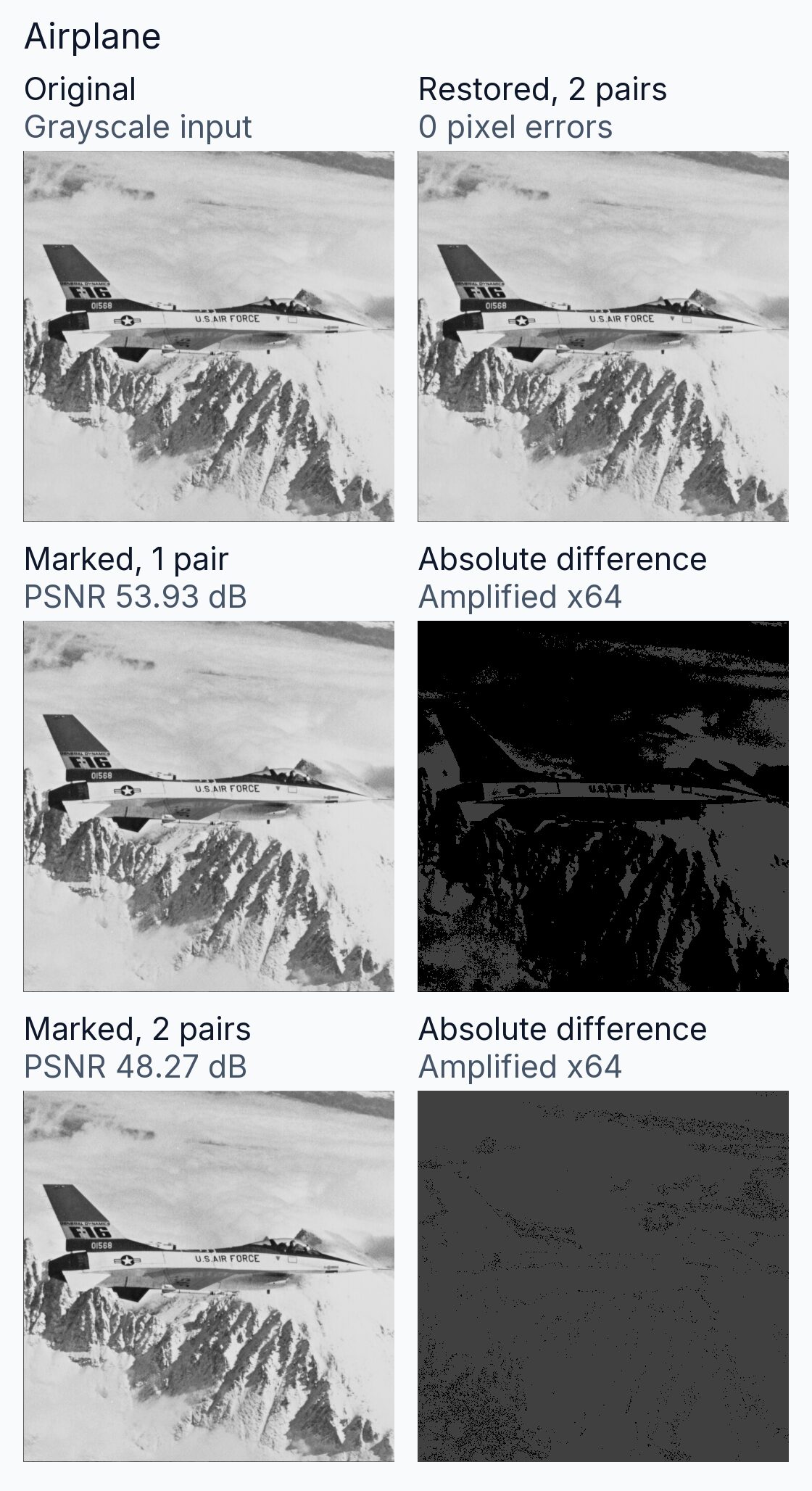
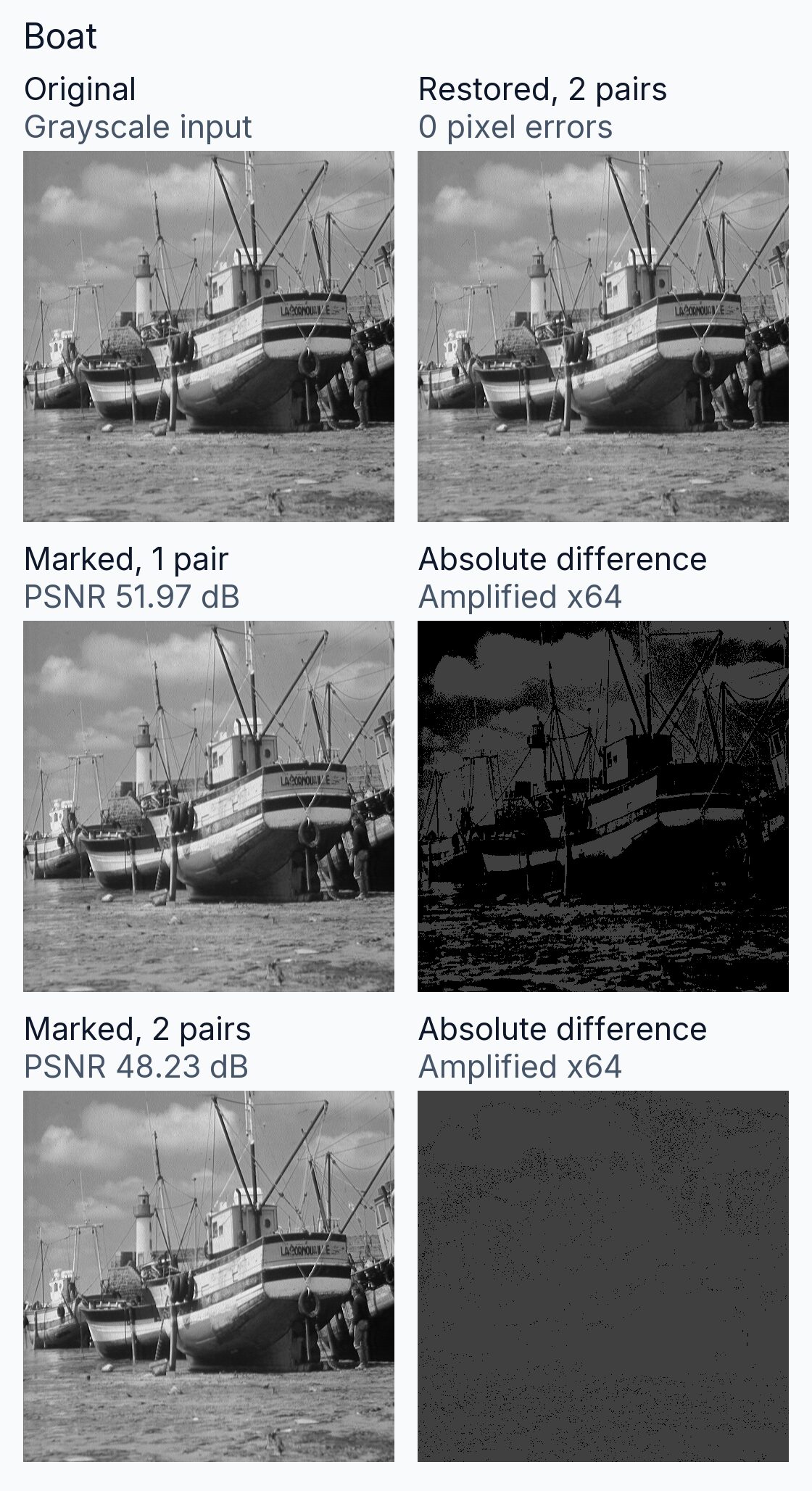
The histogram chart counts the original grayscale pixels. Its point lists identify the peak and zero or minimum for each pair. Boat’s two-pair case uses an occupied minimum and reserves 81 bits for its restoration records.
We measured the following capacities and PSNR values. PSNR is rounded to two decimal places.
| Case | Net bits | PSNR |
|---|---|---|
| Airplane, 1 pair | 8,312 | 53.93 dB |
| Airplane, 2 pairs | 16,040 | 48.27 dB |
| Boat, 1 pair | 5,796 | 51.97 dB |
| Boat, 2 pairs | 11,392 | 48.23 dB |
All four cases restored every pixel and recovered every message bit exactly. Each marked pixel differed from its original by at most one brightness level. The two-pair outputs carried additional message bits and changed additional pixels in each image.
| Item | Setting |
|---|---|
| Random bits | Fixed starting value: 200603 |
| Python version | 3.11.15 |
| Preparation | Converted to 8-bit grayscale; no resizing |
| Scan | Left to right, top to bottom |
| Minimum record | Value: 8 bits; count: 19; position: 18 |
| Storage | Lossless grayscale image files |
Conditions and limits
Recovery requires intact marked pixel values, the pair parameters and the same scan order. An occupied minimum also needs its saved pixel positions. Section II-F identifies the exactly flat histogram as a failure case. The authors qualify their multiple-pair selection as potentially suboptimal for capacity relative to image quality.
Our test used lossless storage, full use of selected peaks and a fixed random stream. Pair parameters traveled separately, and position records used a fixed encoding. We tested no compression, cropping, noise, authentication system or protection against message tampering.
Implementation details
For the multiple-pair test, minima are selected in the lower and upper brightness halves. Neighboring peaks define disjoint shift ranges. Minimum searches exclude brightness endpoints; the single-pair search also excludes values adjacent to the global peak. The global peak is the darkest value with the largest count. Other peak ties favor the brighter value. Minimum ties favor the value closest to the global peak, then the darker value. The test settings include the position-record encoding used by our implementation.
References
- Ni, Z., Shi, Y.-Q., Ansari, N., and Su, W. (2006). Reversible Data Hiding. IEEE Transactions on Circuits and Systems for Video Technology, 16(3), 354-362. DOI: 10.1109/TCSVT.2006.869964. Full text.
- University of Southern California, Signal and Image Processing Institute. USC-SIPI Image Database, Miscellaneous volume: Airplane (4.2.05) and Boat (boat.512). Image catalog.
- Our re-implementation code and numeric results: GitHub, ni-2006-histogram-shifting.