StegaStamp: Invisible Hyperlinks in Physical Photographs (Tancik et al., 2020)
StegaStamp hides a hyperlink identifier inside a photograph through changes to its pixels. The encoded photograph can be printed or displayed on a screen, then photographed by a camera. A detector finds the photograph, and a decoder recovers its identifier for an information lookup. Matthew Tancik, Ben Mildenhall and Ren Ng train the encoding and decoding networks together using simulated distortions from printing, display and photography. The authors frame the task as connecting physical photographs to internet resources while retaining the photograph’s appearance. Tancik et al., StegaStamp: Invisible Hyperlinks in Physical Photographs (2020), arXiv v2.
Why encode a hyperlink into a printed photo at all?
The authors want a camera pointed at an ordinary photograph to retrieve associated information. Section 1 gives examples including produce information beside a market photograph, faculty details linked from a photo directory, and product information associated with digital billboards. The photo itself carries the identifier, so the system can retrieve the link after the image moves from a digital file to a physical surface.
The encoded data is a lookup key for a hyperlink, rather than the characters of a complete web address. A service assigns a unique bitstring to the destination. After camera capture, the recovered key selects the associated resource. The authors motivate hidden encoding as a way to retain the image without adding a visible barcode. Their training objective therefore combines two requirements: recover the key after physical transmission and limit changes to the visible image.
What networks does StegaStamp train?
Encoder and decoder cooperate to carry a binary message through an image. The encoder receives the cover and message and predicts an RGB residual. Adding that residual to the cover creates the StegaStamp. The decoder receives an encoded or distorted image and predicts the message. Its spatial transformer network, or STN, estimates a geometric correction before the message-reading layers.
Two further networks have separate roles. A critic learns a cover-versus-encoded distinction and supplies an image-quality training signal. A BiSeNet detector is fine-tuned to locate StegaStamps in camera frames. The detector produces candidate regions for rectification before decoding. The differentiable perturbation module sits between encoder and decoder during training; its transformations simulate the physical channel. Figure 1 presents the encode, capture, detect and decode flow. Sections 4.2–4.4 describe the STN, detector and critic.
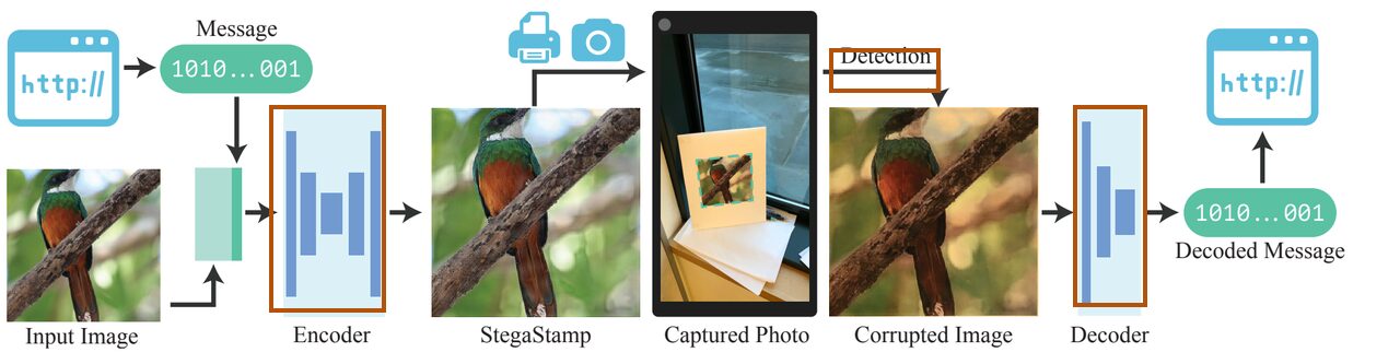
Tancik et al. (2020), Figure 1. Highlights locate encoding, detection and decoding.
How do the 100 bits enter the image?
Section 4.1 projects the binary message through a fully connected layer into a 50×50×3 tensor. Upsampling expands this message representation to 400×400×3. The authors state that preprocessing the message this way aids convergence. Concatenation with the RGB image gives the six input channels listed in supplement Table 5.
The U-Net reduces spatial size while increasing feature channels, then upsamples features and concatenates corresponding earlier features. The final skip combines the first convolution, the last upsampled features and the fused image-message input. Table 5 applies ReLU after every layer except the final residual layer. The residual is added to the original image rather than replacing it with a reconstructed image.
The diagram uses the saved export’s layer shapes. Paired upsampling and convolution stages have matching output sizes; the final linear layer produces three residual channels. Spatial dimensions are height × width × channels, with the batch omitted.
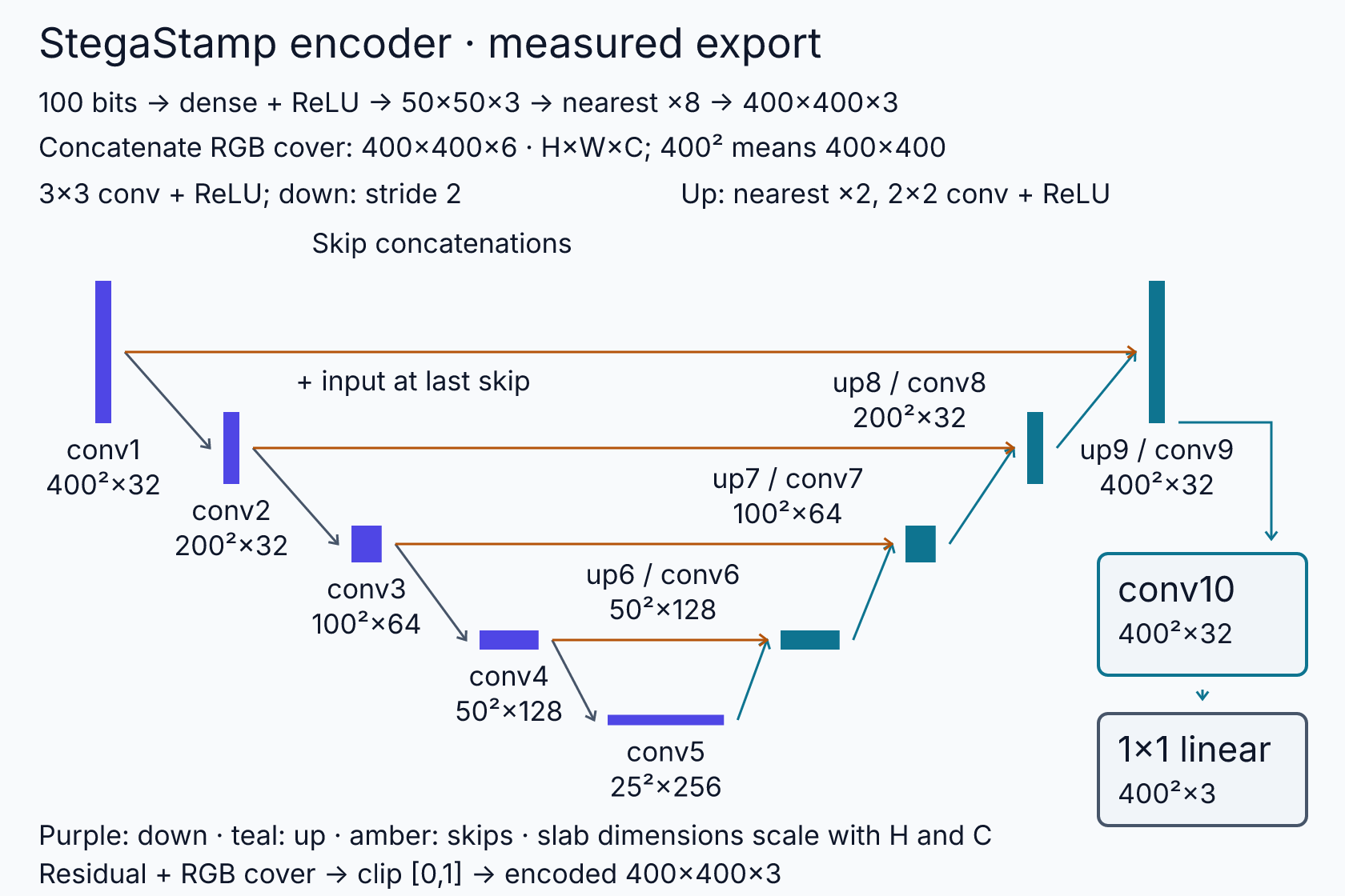
Saved export architecture from network_layers.csv; slab height scales with spatial size and width with channel count.
How does the decoder handle geometry?
A photograph of a planar image changes its apparent shape and sampling. The external detector first rectifies a candidate region. Section 4.2 then uses an STN inside the decoder to accommodate remaining small geometric changes introduced by capture and rectification. The STN predicts an affine transform; it is separate from the detector’s projective homography.
Supplement Table 6 describes a localisation network with three strided convolutions, flattening and dense layers. Six outputs specify the affine warp. A differentiable sampler transforms the image before a second convolutional stack reads the bits. Dense layers and a sigmoid produce a prediction for each message bit. Cross-entropy supervises those predictions during training.
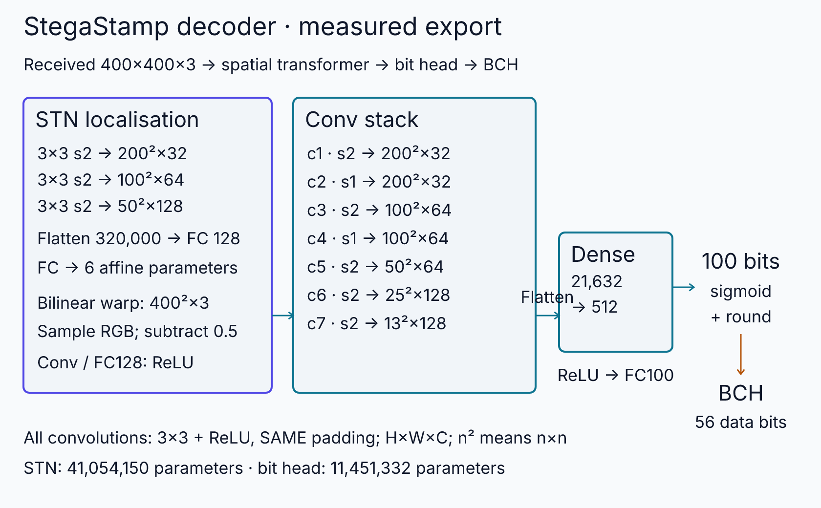
Saved export architecture; the transform corrects the decoder input before message prediction.
In our worked example on Boat, we measured 100/100 raw bits from the clean encoded PNG. A separate 5° rotation gave 90/100 and failed exact recovery after BCH. The specified perspective warp gave 100/100 and recovered Stega!!. Rotation used bicubic sampling and black fill; perspective used bilinear sampling and white fill.
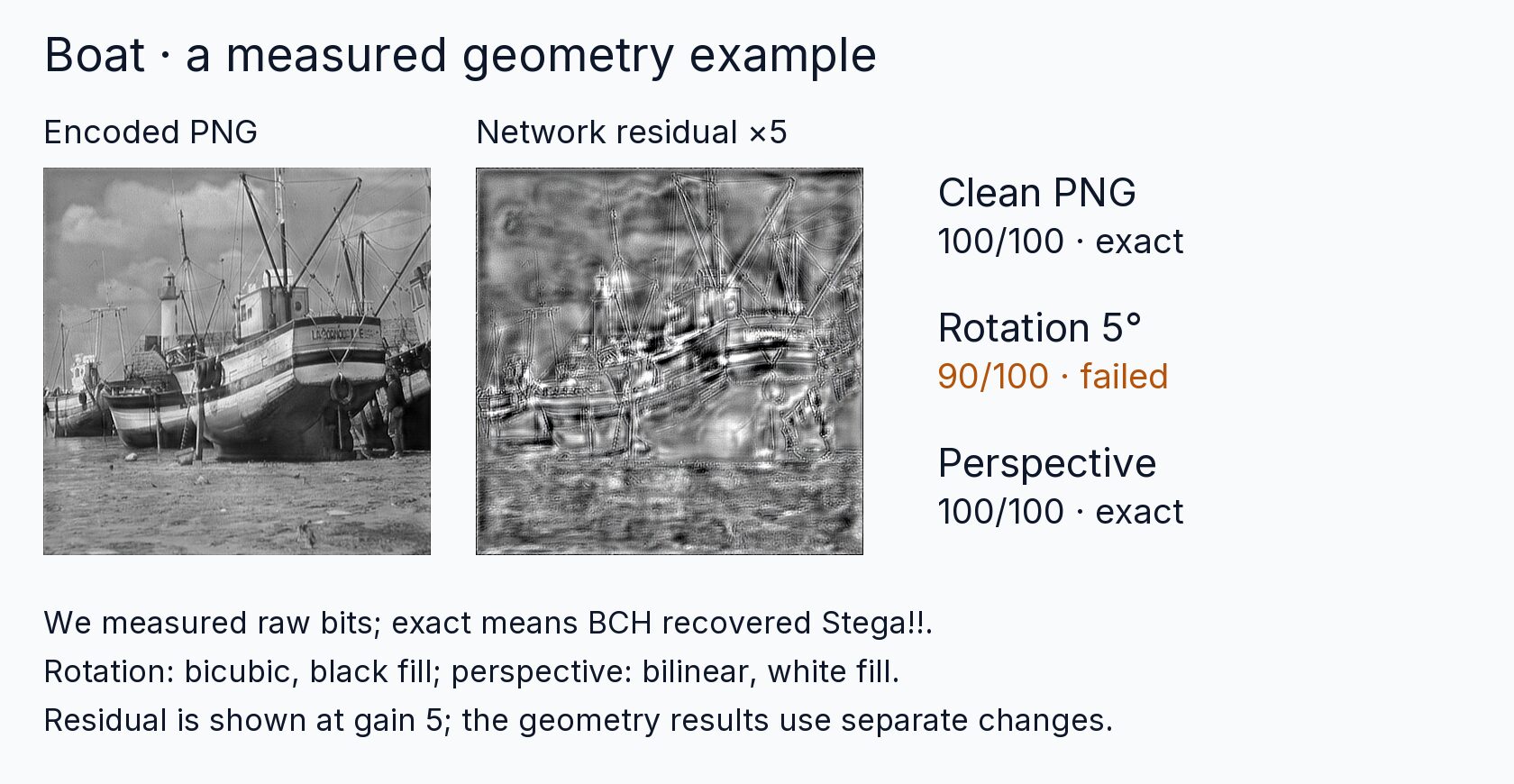
We measured these separate changes to the encoded Boat image; residual display is clip(0.5 + 5×residual, 0, 1).
Which image changes are simulated during training, and why?
Section 3 inserts differentiable changes between encoding and decoding. Perspective warping models a camera viewing a planar surface from another position. Motion and defocus blur model camera motion and inaccurate focus. Colour transformations approximate printer/display gamut, exposure, white balance and colour processing. Gaussian noise models imaging noise under the authors’ stated non-photon-starved conditions. JPEG approximation models lossy camera-image storage.
| Change | Paper’s training range | Operation |
|---|---|---|
| Perspective | Corners up to ±40 pixels, ±10% | Solve homography; bilinear resampling |
| Motion blur | Line width 3–7 pixels; random angle | Convolution with line kernel |
| Defocus blur | Gaussian σ=1–3 pixels | Gaussian convolution |
| Colour | RGB offsets [−0.1, 0.1]; desaturation interpolation | Constant across the image |
| Brightness / contrast | m∈[0.5, 1.5], b∈[−0.3, 0.3] | mx+b; clip channels to [0, 1] |
| Noise | Gaussian σ∈[0, 0.2] | Additive imaging noise |
| JPEG approximation | Quality [50, 100] | Differentiable quantization surrogate |
Source: Tancik et al. (2020), Sections 3.1–3.5.
Figure 3 presents these families as an image perturbation pipeline.
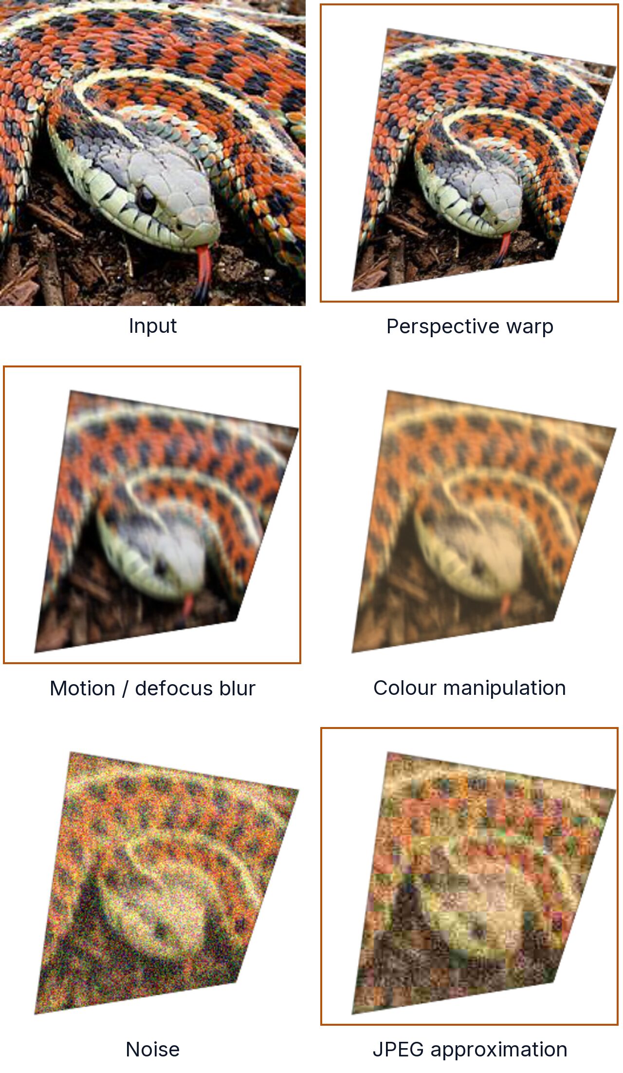
Tancik et al. (2020), Figure 3. Highlights mark perspective warp, blur and JPEG approximation.
How can JPEG compression support gradient-based training?
JPEG transforms each 8×8 block into discrete cosine transform coefficients and quantizes them by rounding. Ordinary rounding interrupts the useful gradient through this part of the encoder-decoder training path. Section 3.5 adopts a differentiable approximation from Shin and Song.
For a coefficient x, the approximation uses x³ when its magnitude is below 0.5 and x otherwise. The paper states that this function has a nonzero derivative almost everywhere. Its training quality is sampled uniformly from 50 to 100. The surrogate supplies a path for message loss to influence encoding through a compression-like operation.
The synthetic ablation separates JPEG from the other perturbations. Section 5.3 reports that the model trained without perturbations fails under JPEG compression, while spatial-only training also gives some JPEG robustness. The authors suggest a shared low-pass effect with blur as a possible explanation for that latter observation.
What does each loss do?
Section 4.4 combines residual L2 regularization, LPIPS perceptual distance, a learned critic term and message cross-entropy. The first three penalize image changes; the message term penalizes incorrect decoded probabilities. LPIPS compares learned image features. The critic is trained with a Wasserstein objective, with critic updates interleaved with encoder-decoder training.
L = lambda_R * L_R + lambda_P * L_P
  + lambda_C * L_C + lambda_M * L_M
The released scripts/base.sh recipe sets the L2, LPIPS, critic and message weights to 2, 1.5, 0.5 and 1.5. Its squared image error is computed in YUV, with channel scales 1, 100 and 100. These values belong to the released recipe; the paper gives the weighted objective and the training rationale.
The paper also strengthens the residual penalty near image edges with a cosine falloff. The authors report distracting edge patterns during training and describe this penalty as their response. In the code, the edge map multiplies the image difference before squaring, so its gain acts inside the squared-error calculation.
Why increase losses and perturbations gradually?
Section 4.4 reports that convergence benefits from beginning with message recovery. Image-loss weights initially remain zero while the decoder learns accurate predictions. The weights then rise linearly. Perturbation strengths also begin at zero; the authors identify perspective warping as the most sensitive perturbation and increase it most slowly.
The released base recipe uses 140,000 steps. Its first 1,500 steps optimize message loss alone. Image-weight formulas use the absolute global step and reach their targets at step 15,000, so enabling the full loss after the initial phase starts partway along those ramps. Perspective reaches full strength at step 10,000. Colour, noise and JPEG defaults ramp over 1,000 steps.
The recipe delays extra edge gain until step 80,000 and ramps it to 10 over 10,000 further steps. Training uses MIRFLICKR images resampled to 400×400 with random binary messages. Released defaults select Adam, learning rate 0.0001 and batches of four.
How is the message protected against bit errors?
Raw bit predictions can contain errors even when much of the message survives. Section 5.4 selects a 100-bit network message and uses BCH error correction to retrieve a 56-bit identifier. Supplement B describes 56 message bits and 40 error-correction bits. The released encoder pads the resulting 96 bits with four zeros to fill the network’s input.
The BCH decoder uses redundancy to recover the original data when the received packet contains a correctable error pattern. The supplement describes successful correction when fewer than five bits are corrupted and filters proposals when correction fails. Exact identifier recovery is therefore a separate outcome from the percentage of raw bits predicted correctly.
The authors choose message length by training separate models and balancing recovery with perceptual quality. They tune image and message losses for at least 95% bit accuracy. Section 5.4 reports more perceptible degradation with 150- and 200-bit messages and fewer possible identifiers with 50 total bits after error correction.
How is a StegaStamp found inside a real photograph?
The decoder operates on a rectified image region. Section 4.3 fine-tunes BiSeNet to segment candidate StegaStamp regions within a wider camera image. Its training data places randomly transformed StegaStamps into high-resolution backgrounds sampled from DIV2K.
At inference, the system takes each proposed region’s convex hull and fits a quadrilateral. A homography maps that quadrilateral to a 400×400 square for decoding. This detector-level localization precedes the decoder’s learned affine correction. The final recovered identifier can then select the linked resource.
The authors describe detection as a bottleneck in their real-world tests. Section 5.1 reports missed detections on some video frames, while noting that their scanning application needs a successful code recovery in only one frame. Section 5.5 states that the current detection framework assumes single, square images.
What happens when training omits perturbations?
The authors train four variants with the same architecture: None, Pixelwise, Spatial and All. Pixelwise includes noise, colour changes and JPEG compression. Spatial includes perspective warp and blur. The comparison changes the distortions encountered during learning, while retaining the encoder-decoder architecture.
Figure 7 sweeps test strength from zero through the maximum seen during training and up to twice that strength. Models trained without spatial perturbations lose recovery under warp and blur. Spatial-only training remains sensitive to colour changes. The authors report that combining both groups yields the strongest recovery across the tested families.
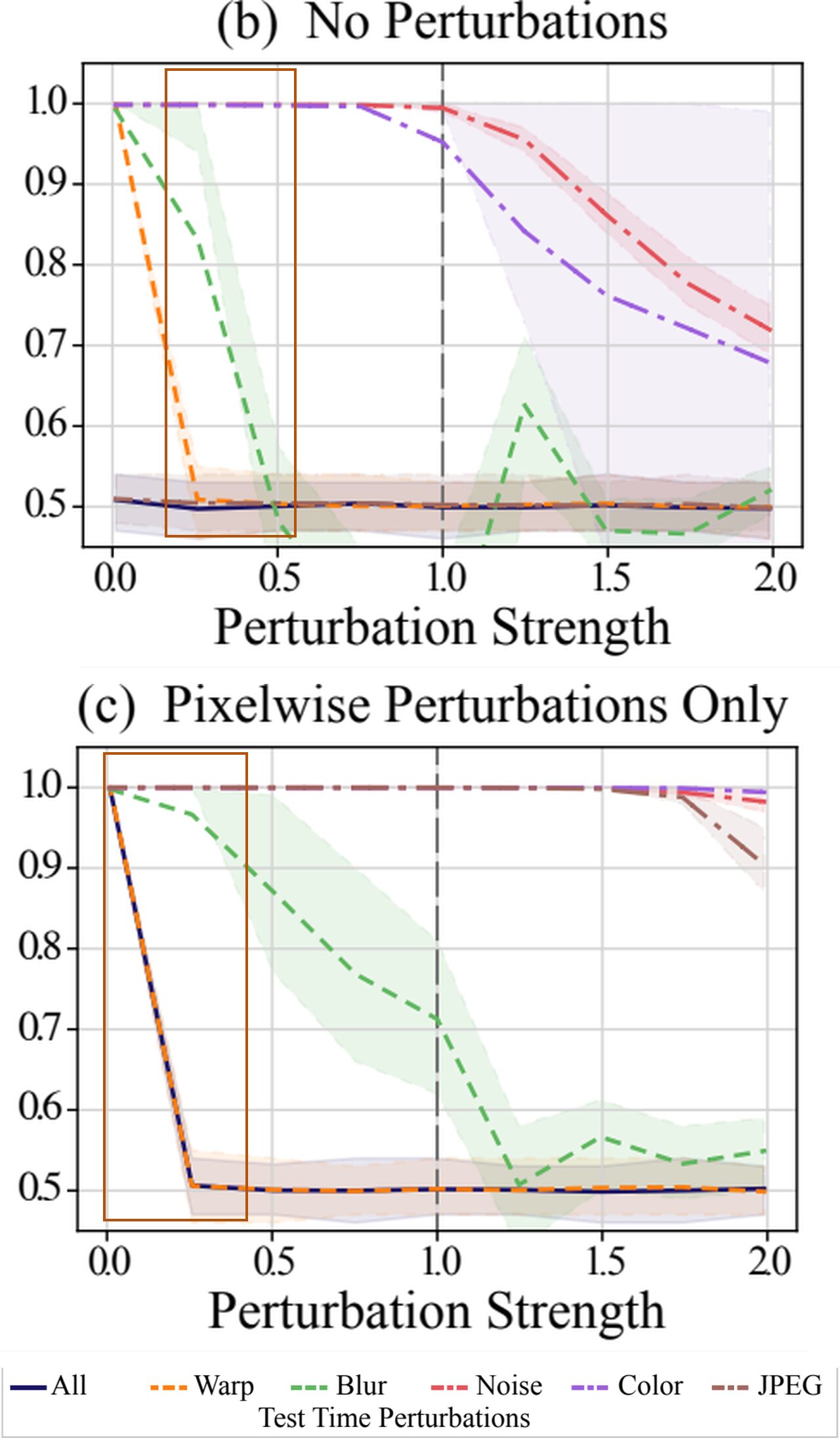
Tancik et al. (2020), Figure 7. Enlarged panels isolate training without spatial changes; the shared legend identifies test perturbations.
All parts of StegaStamp
Joint training sends the cover and packet through the encoder, simulated image changes and decoder. Message loss connects decoded predictions to the original bits. L2/YUV, LPIPS and critic losses constrain the encoded image. The critic is trained separately within that procedure. At inference, printing or display and camera capture replace the simulated channel. BiSeNet proposes a region, quadrilateral rectification creates a square input, and the decoder predicts packet bits for BCH recovery.
What experiments did the authors run?
The authors evaluate physical capture, baseline methods, training ablations, message length, image quality, detection and partial occlusion.
Controlled printer, screen and camera combinations
Section 5.2 selects 100 ImageNet source images, disjoint from training, with random 100-bit messages. Five additional encodings reuse one source with different messages, producing 105 test images. Fixed lighting, a display rig and tripod-mounted cameras control capture. Each photograph is manually cropped and rectified before decoding. The full set has 1,890 captures across 18 combinations and mean bit accuracy 98.7%.
Printers are HP LaserJet Enterprise CP4025, HP LaserJet Pro M281fdw and Xerox 700i Digital Color Press. Screens are Dell ST2410, MacBook Pro 15-inch and iPhone X. Capture devices are Logitech C920, Google Pixel 3 and Canon 5D Mark II. Factory calibration settings are retained. Table 1 reports raw-bit accuracy percentiles and means, with the enterprise-printer webcam mean 95.9% and DSLR screen means 99.8%.
| Camera / medium | 5th (%) | 25th (%) | Median (%) | Mean (%) |
|---|---|---|---|---|
| Webcam / enterprise printer | 88 | 94 | 98 | 95.9 |
| Webcam / consumer printer | 90 | 98 | 99 | 98.1 |
| Webcam / pro printer | 97 | 99 | 100 | 99.2 |
| Webcam / monitor | 94 | 98 | 99 | 98.5 |
| Webcam / laptop | 97 | 99 | 100 | 99.1 |
| Webcam / cellphone screen | 91 | 98 | 99 | 97.7 |
| Cellphone / enterprise printer | 88 | 96 | 98 | 96.8 |
| Cellphone / consumer printer | 95 | 99 | 100 | 99.0 |
| Cellphone / pro printer | 97 | 99 | 100 | 99.3 |
| Cellphone / monitor | 98 | 99 | 100 | 99.4 |
| Cellphone / laptop | 98 | 99 | 100 | 99.7 |
| Cellphone / cellphone screen | 96 | 99 | 100 | 99.2 |
| DSLR / enterprise printer | 86 | 96 | 99 | 97.0 |
| DSLR / consumer printer | 97 | 99 | 100 | 99.3 |
| DSLR / pro printer | 98 | 99 | 100 | 99.5 |
| DSLR / monitor | 99 | 100 | 100 | 99.8 |
| DSLR / laptop | 99 | 100 | 100 | 99.8 |
| DSLR / cellphone screen | 99 | 100 | 100 | 99.8 |
Source: Tancik et al. (2020), Table 1.
Comparisons and physical perturbation ablations
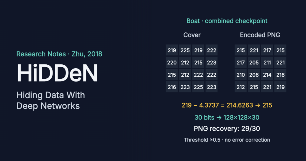
The cellphone-camera/consumer-printer condition compares StegaStamp variants, Baluja, HiDDeN and Light Field Messaging, or LFM. Supplement C retrains Baluja with upscaled binary grids. HiDDeN retains 30 bits in native 128×128 images because the authors observed degraded performance at 100 bits and larger size. LFM averages nine block predictions per bit. Its additional screen condition uses cellphone capture of a cellphone screen.
The supplement reports mean accuracy and a channel-capacity-derived bits-per-megapixel measure to account for message and image sizes. All reaches 0.99 mean accuracy; Spatial reaches 0.89. LFM’s screen and print means are 0.93 and 0.61.
| Method / training | Mean accuracy | Bits/MP |
|---|---|---|
| Baluja | 0.51 | 0.5 |
| HiDDeN | 0.65 | 125 |
| LFM, printed | 0.61 | 287 |
| LFM, screen | 0.93 | 1109 |
| StegaStamp, None | 0.49 | 0.1 |
| StegaStamp, Pixelwise | 0.51 | 0.2 |
| StegaStamp, Spatial | 0.89 | 318 |
| StegaStamp, All | 0.99 | 571 |
Source: Tancik et al. (2020), Table 3.
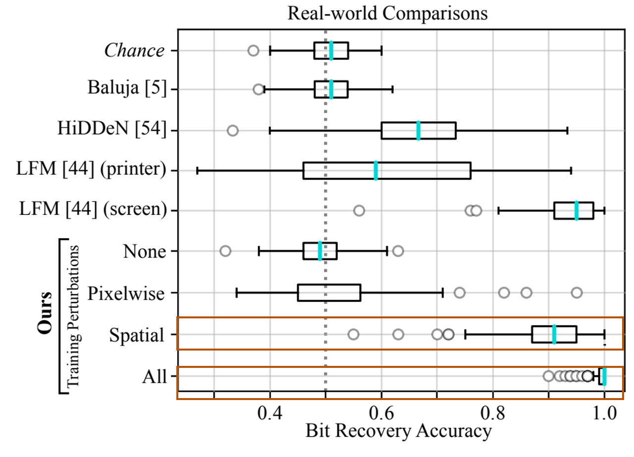
Tancik et al. (2020), Figure 6. Highlights identify the Spatial and All distributions.
Synthetic strength sweeps
Section 5.3 evaluates the four training variants with warp, blur, noise, colour, JPEG and their combination. Strength 1 is the largest training value; strength 2 doubles the parameterized degradation. Figure 7 plots mean accuracy and interquartile bands. Its caption specifies 100 random images and messages; Section 5.3 instead states 1,000 images. The paper reports immediate sensitivity to resampling for the None and Pixelwise variants, and sensitivity to colour for Spatial. These are separate trained models, not modules disabled during decoding.
Message length and image quality
Section 5.4 trains separate models for 50, 100, 150 and 200 bits. Table 2 averages image quality over 500 images. The 100-bit model has 28.50 dB PSNR, 0.905 SSIM and 0.101 LPIPS. PSNR and SSIM increase with similarity; LPIPS decreases.
| Metric | 50 bits | 100 bits | 150 bits | 200 bits |
|---|---|---|---|---|
| PSNR (dB) | 29.88 | 28.50 | 26.47 | 21.79 |
| SSIM | 0.930 | 0.905 | 0.876 | 0.793 |
| LPIPS | 0.100 | 0.101 | 0.128 | 0.184 |
Source: Tancik et al. (2020), Table 2.
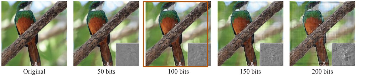
Tancik et al. (2020), Figure 8. The highlight identifies the 100-bit image and residual inset.
Supplement C separately compares image quality between methods. It includes HiDDeN both at native size and after bicubic upsampling to 400×400. Its StegaStamp row reports 27.25, 0.927 and 0.194 for PSNR, SSIM and LPIPS.
| Method | PSNR (dB) | SSIM | LPIPS |
|---|---|---|---|
| Baluja | 24.61 | 0.926 | 0.256 |
| HiDDeN, native | 31.07 | 0.940 | 0.070 |
| HiDDeN, upsampled | 24.55 | 0.775 | 0.202 |
| LFM | 20.89 | 0.910 | 0.315 |
| StegaStamp | 27.25 | 0.927 | 0.194 |
Source: Tancik et al. (2020), Table 4.
Handheld video, detector behaviour and occlusion
Section 5.1 uses handheld cellphone video in indoor and outdoor environments, with consumer-printed StegaStamps. Figure 4 displays detected quadrilaterals and bit percentages, including 98%, 99% and 100%. The authors report high decoding accuracy when the bounding rectangle is accurately located, with some missed video-frame detections.
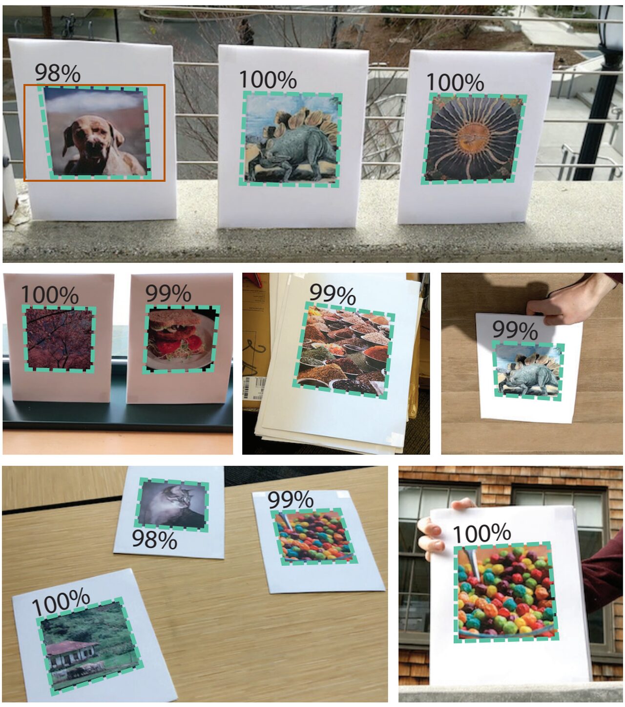
Tancik et al. (2020), Figure 4. Highlighted quadrilateral marks a detected print.
Figure 5 places objects over parts of printed images and labels raw-bit accuracies of 97%, 99% and 97%. The authors state that occlusion robustness was not explicitly trained. Supplement B’s first video filters detections below 70% bit accuracy; its second uses BCH and displays successful corrected messages. The authors’ limits include visible residuals in some low-frequency image regions and the detector’s single-square-image assumption.
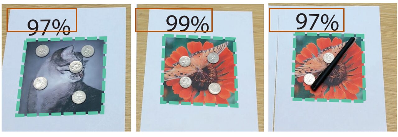
Tancik et al. (2020), Figure 5. Highlights mark the reported bit percentages.
Our test: can the saved message survive digital image changes?
Setup
We used a community mirror of the encoder-decoder SavedModel with a fixed secret. Our code and numeric results are on GitHub.
| Setting | Value |
|---|---|
| Weights | Community mirror Gu-f of the official SavedModel; original identity unverified; graph, variable shard and index byte-identical to a second independent mirror copy |
| Runtime | TensorFlow 1.15.5; CPU; float32 |
| Images | USC-SIPI Airplane and Boat; RGB, fitted to 400×400 |
| Secret | Stega!!; BCH packet with zero padding |
| Seed | 20231130; fixed offsets per operation and image |
| Repeated runs | run1/run2: 15 result/settings/array files byte-identical; timings excluded |
| Serialization | Clip to [0, 1], multiply by 255, truncate to uint8; reopen PNG for changes |
| Combined noise maximum | Standard deviation 0.02, from the code setting |
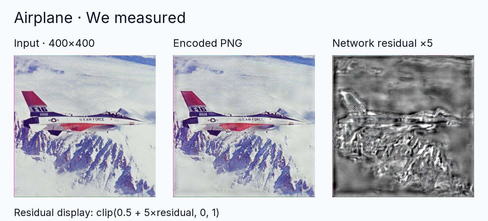
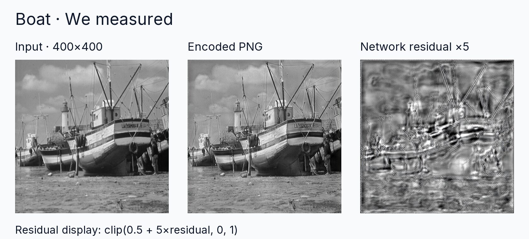
We measured the displayed inputs and encoded PNGs. Residual display is clip(0.5 + 5×network residual, 0, 1).
Quality
We measured RGB PSNR of 28.9471 dB and SSIM 0.911483 for Airplane, and 28.9556 dB and 0.907496 for Boat. The reference is the fitted input; the encoded image is the serialized PNG. SSIM uses a seven-pixel window, uniform weights, sample covariance and the RGB-channel mean. Clean PNG decoding recovered 100/100 raw bits and the exact secret from each image.
Single changes
Every change begins with the encoded PNG. JPEG uses qualities 90, 70, 50 and 30 with 4:2:0 subsampling. Gaussian blur uses σ=1 and 2 with reflected boundaries; Gaussian noise uses standard deviations 0.02 and 0.05 with clipping. Brightness, contrast and saturation use the factors labelled in the charts. Hue shifts by 0.05 turn. Resize halves each side before restoring the working dimensions with Lanczos interpolation.
We measured 92/100 and 90/100 raw bits after 5° rotation on Airplane and Boat; exact recovery failed for both. At 10°, the counts were 63/100 and 56/100. The central crop retains 90% of each side and resizes back; Airplane returned 88/100 with failed exact recovery, while Boat returned 100/100 with exact recovery. Horizontal flips returned 55/100 and 57/100 with failures. Perspective used destination corners (20,15), (380,0), (399,380), (10,399), bilinear sampling and white fill, yielding exact recovery on both images. Amber rings mark failed exact-secret recovery after BCH.
Combined changes
Each draw applies perspective warp, blur, noise, contrast plus RGB/brightness offsets, desaturation and the differentiable JPEG surrogate. Draws sample full configured ranges: corner bound floor(400×0.1×U[0,1)); blur is Gaussian, motion or identity; contrast [0.5,1.5], RGB offsets [−0.1,0.1], brightness [−0.3,0.3], desaturation [0,1] and JPEG quality [50,100]. Gaussian blur samples σ∈[1,3]. The blur mixture selects Gaussian and motion with probability 0.25 each and identity with probability 0.5. This chain directly warps the saved encoded image; NumPy supplies deterministic random draws.
We measured exact recovery on 17/20 Airplane draws and 20/20 Boat draws. Mean raw-bit counts were 98.70/100 and 99.90/100, with minima 91/100 and 99/100. Airplane failed on draws 3, 10 and 11, with raw counts 94, 94 and 91. Boat recovered the exact secret on every draw. The chart plots every draw on a shared raw-bit axis.
Conditions and limits
Physical decoding requires a localized and rectified photograph, the corresponding decoder and successful packet correction. The authors’ detector assumes a single square image region and can miss individual video frames. Their controlled device experiment uses manual rectification.
Our measurements cover digital changes to two fixed images carrying one fixed secret. They include neither print/camera capture nor BiSeNet detection. The weights come from a community mirror; agreement with a second copy establishes byte identity between those copies, while the original release’s identity remains unverified. The combined chain uses the saved encoded image, explicit random seeds and the stated interpolation and boundary settings.
What came after
TrustMark (Bui et al., 2023) benchmarks StegaStamp and develops watermarking with resolution scaling and watermark removal. WAVES (An et al., 2024) includes StegaStamp in a benchmark of watermark detection and identification under image distortions, regeneration and adversarial attacks; the authors’ benchmark page presents its StegaStamp results.
Implementation details
The saved export’s measured sizes, excluding the training critic and separate detector, are:
| Module | Parameters | Input → output |
|---|---|---|
| Secret path | 757,500 | 100 → 50×50×3 → 400×400×3 |
| Encoder U-Net / residual | 991,747 | 400×400×6 → 400×400×3 |
| Decoder STN | 41,054,150 | 400×400×3 → 6 affine values → warped RGB |
| Decoder bit head | 11,451,332 | Warped RGB → 13×13×128 → 21,632 → 512 → 100 |
| Total | 54,254,729 | Encoder and decoder deployment graph |
Table 5 and the export use six encoder input channels; Section 4.1 says four. The export follows conv10→residual, matching Table 5. Pinned models.py computes conv10 but returns residual(conv9). The export’s SAME-padded decoder reaches 13×13×128 and flattens to 21,632; Table 6 lists 20,000. STN localisation flattens to 320,000 in both.
The export samples uncentered RGB in its STN and subtracts 0.5 afterward. The pinned source subtracts 0.5 before sampling. The paper describes a max-pooling critic; the source uses spatial averaging. Section 3.4 specifies noise maximum 0.2; train.py sets 0.02.
The source archive is pinned to c984446048b826587ca1875027b0a1dc1885fb30. The Gu-f mirror is pinned to d95ea307c73410c96557200656d2e0a59574eedb; the second mirror is pinned to 84e34ef46e27b5fe847d474853a133b730a1ec03. Original identity is unverified. SHA-256 digests of the matching model files are:
saved_model.pb
42c4be663021a1d98f82eed425ac6643aa149d57e8bb5a60be2247e19937f095
variables.data-00000-of-00001
1ca5cd940906f57454fcf3d05d4f81edd87066903f7ced2ba57399614bca3bf0
variables.index
8c038f8fa37dba430c59dd91a654f2aedffff27acf0efed657d2d15f46d5149c
Our code and numeric results include tensor shapes, layer parameters, packet bits, seeds, per-change settings and both result runs. The combined sampler uses a 7×7 channel-diagonal blur kernel with zero padding; its motion component samples angle [0,2π), transverse σ∈[0.25,1] and Manhattan threshold [3,3.1]. Airplane’s draw seed is the base seed plus its zero-based draw index; Boat adds 1,000. No residual-strength sweep is exposed by the saved serving interface.
References
- Tancik, M., Mildenhall, B., and Ng, R. StegaStamp: Invisible Hyperlinks in Physical Photographs, arXiv:1904.05343v2, 2020; main paper and supplement, Tables 1–6 and Figures 1–9.
- Tancik et al. Official source snapshot, including
models.py,train.py,encode_image.pyandscripts/base.sh; MIT license. - Gu-f SavedModel mirror and independent second mirror copy; original identity unverified.
- USC-SIPI Image Database, miscellaneous volume, Airplane and Boat; source terms.
- Bui, T., Agarwal, S., and Collomosse, J. TrustMark: Universal Watermarking for Arbitrary Resolution Images, 2023.
- An, B., et al. WAVES: Benchmarking the Robustness of Image Watermarks, ICML 2024; benchmark results.